Introduction
In lab 1, we explored the mass transfer rate from the donor, but did not evolve the accretor. In lab 2, we explored the accretion up to the helium flash on the accretor, for a fixed accretion rate. Now, we want to see what would happen to the accretor if we use the time-dependent mass transfer rate from lab 1. Normally, you would evolve both the donor and accretor together in the binary module, by setting evolve_both_stars = .true. in the binary inlist. This would take too long for the MESA summer school. So instead, we will implement this in the star module. We will take the history file from lab 1, read in the mass transfer rate, and add this to the accretor using ./src/run_star_extras.f90.
Lab Instructions
For this lab, we will use run_star_extras.f90 to interpolate the Mdot from Lab 1 and ultimately measure a more-realistic thickness of the Helium shell (as compared to our values from Lab 2)
Some helpful links
link to the Google spreadsheet of options
link to the GitHub repo (general link)
link to the MESA documentation
Task 0. Copy Files
This lab will combine the work we have done so far in labs 1 and 2. To ease the set up process, we will be continuing from the end point of Lab 2. Make a copy of your directory from Lab 2 (excluding the ./photos and ./LOGS folders) then copy over the ./LOGS1/history.data file generated in Lab 1 (NOT the binary_history.data file). If you didn’t complete Labs 1 or 2 for any reason, you may instead download the Lab 2 solutions from the GitHub repo. A selection of history files for Lab 1 are in the GitHub repo (direct link), as well. They are formatted in folders labeled as < donor type >< donor mass >< donor entropy >< accretor mass >< binary period>.
Additionally, we have provided a more scaffolded approach to this lab, with a partially annotated version of ./src/run_star_extras.f90 available from the GitHub repo here. Download this file and place it in the ./src/ folder of your working directory.
inlist_project
inlist_pgstar
inlist
nco.net
history.data
cowd_< >M_Tc2e7.mod
tables_hashimoto/
src/
make/
mk
clean
re
rn
Task 1. Writing the interpolation Code
In this task, we will be writing an interpolation script in run_star_extras.f90 that does the following:
- Initializes new variables
- Opens a history file
- Skips through the history file header
- Sets a proper file format
- Reads in the history file contents
- Limits the timestep,
dt - Interpolates Mdot, linearly
- Sets the Mdot value of the next timestep
Don’t worry if this seems like a lot! We will be going through this step-by-step and remember the solution can be found here, if you get stuck. We recommend looking at the solution frequently throughout this lab!
Recall the control flow in MESA (below), that is, which routines get called at which points during a MESA run. Identify which subroutine (or function) would need to be modified in order to interpolate the varying mdot produced in Lab 1 and find that routine in run_star_extras. Remember, this interpolation will need to be completed before MESA attempts to solve the star’s state.
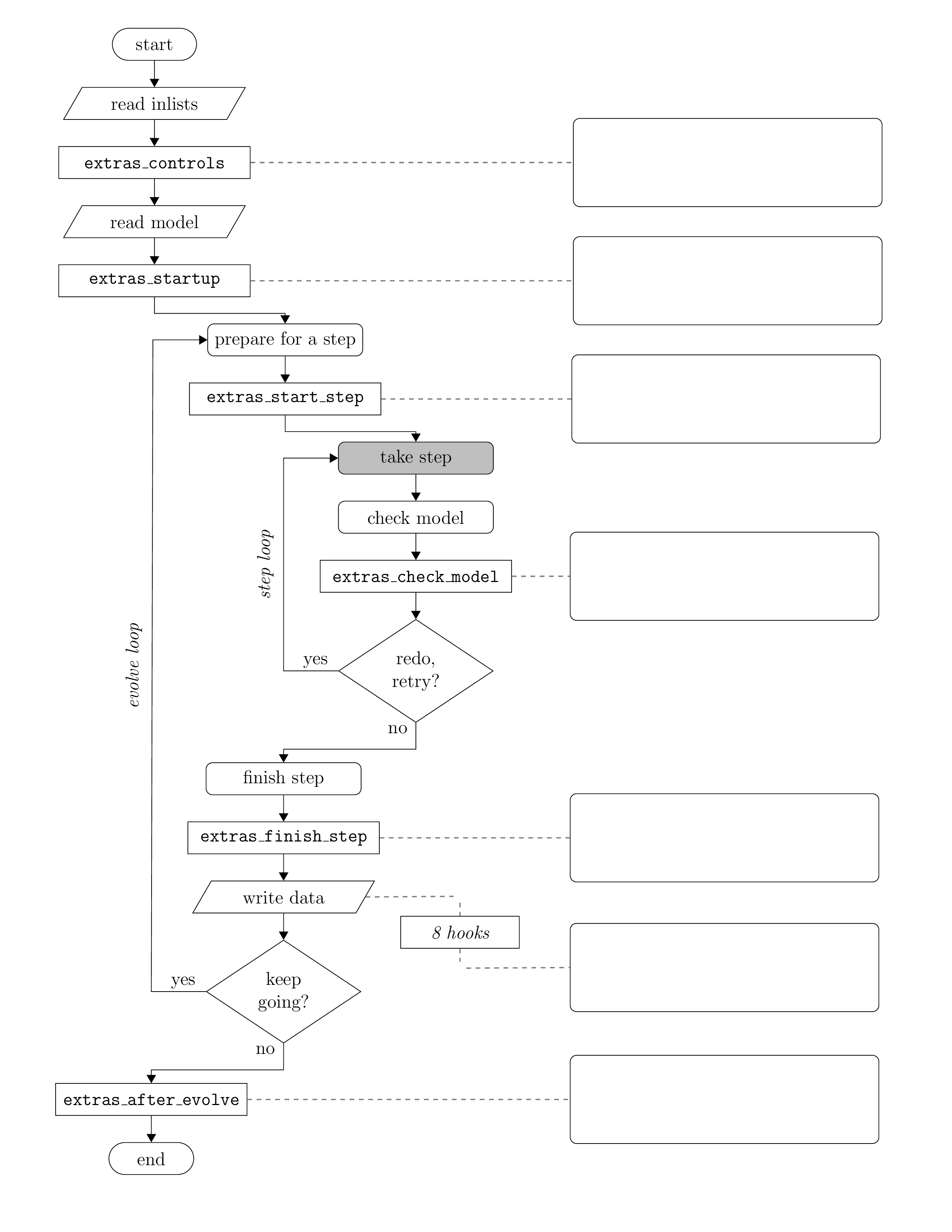
Hint (click here)
We will make the following changes in extras_start_step
Look through the subroutines in run_star_extras and observe their general form. A subroutine (or function) is named, variables are declared, the error status is set and checked, the “stuff” of the subroutine occurs, then the subroutine ends. Since we have just identified the function we will be modifying, let’s take a look at the variables we will need. Open the donor history file, history.data and take a look around. How many columns are before the mdot (log_abs_mdot)? How many rows before our relevant data begins?
If all is according to plan, you should notice six (6) labeled columns before log_abs_mdot, and six (6) header rows before data begins. Below is an example of the structure of this history.data file, note that the particular data may vary.
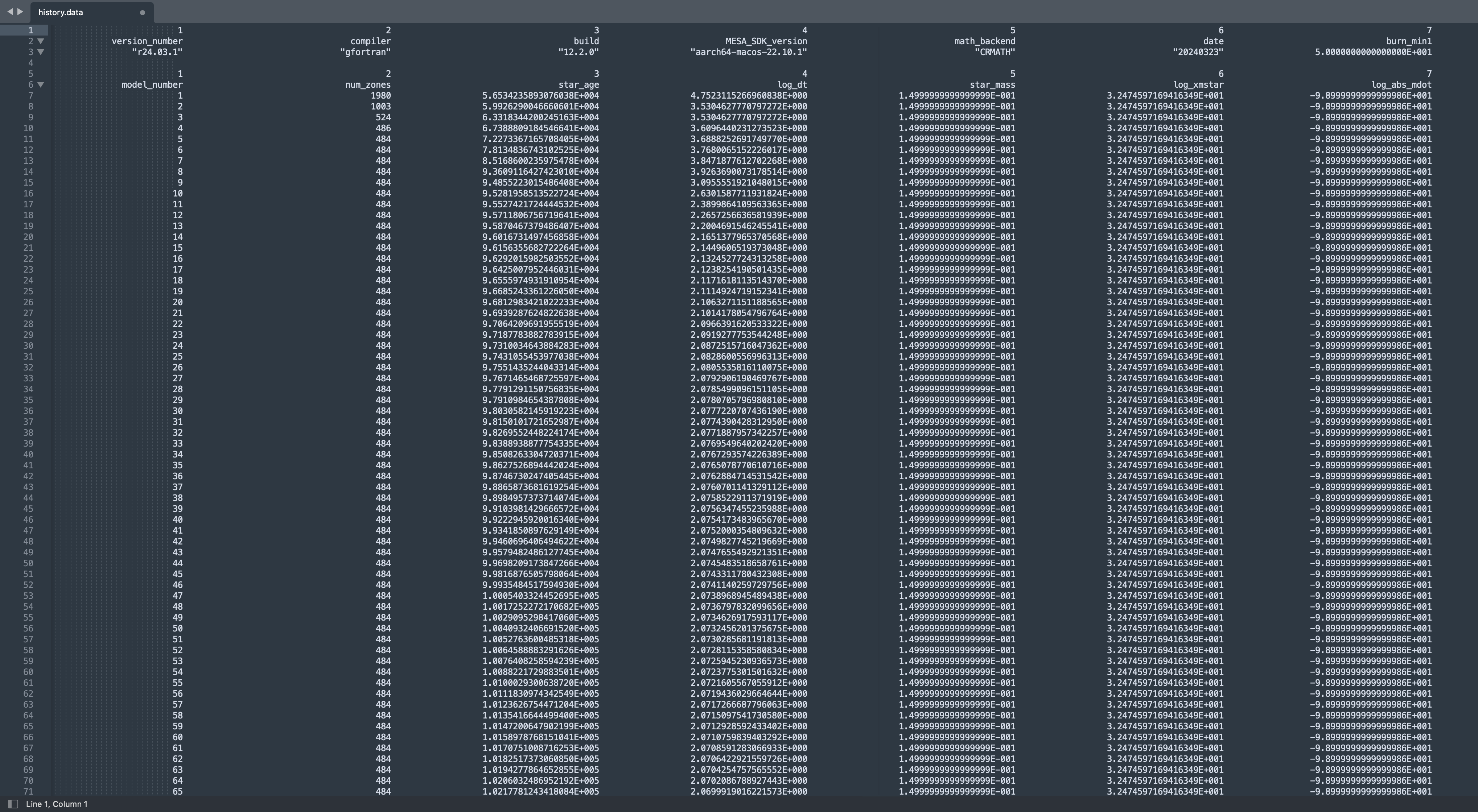
When opening the file, our interpolation function will read the contents row by row. This allows us to easily skip the header section (we will worry about this later), but we CANNOT skip columns. On a given row, the interpolation function must read the columns in order. So, although we will only need star_age, log_dt, and log_abs_mdot, we still need a place to dump the irrelevant data that is intertwined. This can be done by establishing placeholder variables that we can set and ignore throughout the calculation. Take note of the order and data type for the columns.
Navigate back to run_star_extras and initialize some variables. We will use a log_Mdot_interp as an intermediate variable in our calculation whose type is real, a counter integer i, and 2 element arrays for star_age, log_dt, and log_Mdot. These declarations should be done above the statement ierr=0, but order does not matter. Remember to format the declarations correctly as type :: name and don’t forget to add in the necessary placeholder variables, placeholder_i and placeholder_r. Note, we are using 2 element arrays for certain data as they allow space for us to store values for both the current and previous timesteps.
An example of variable initialization is below. Feel free to read more about Fortran arrays here. Another good resource for Fortran90 basics is this. Feel free to explore these resources at your own pace after the Summer School.
! Add Variables
integer :: i
real(dp), dimension(2) :: star_age
real(dp) :: log_Mdot_interp
Hint (click here)
The types used are integer, real(dp), and real(dp), dimension(2)
Feel free to check out the solutions if you are stuck!
Now that we have wrangled our variables, we need to tell Fortran to open the history.data file. Use your profound access to all of human knowledge to find the function that connects an external file to an input/ouput unit (ie. Google it or control-F here). Set unit=33, file = '< local path to history.data >', and action='read'. Remember to write this after the error check, beneath extras_start_step = 0.
- Note: The unit refers to a Fortran logical unit, the interface for data transfer in Fortran. The unit number we chose (33) was largely arbitrary and chosen for consistency, not necessity. The only rule here is that the value needed to be a nonnegative integer.
Hint (click here)
!! open file

open(unit=33, file='history.data', action='read')
With the interface to the file established, let’s make sure to skip through that header that we saw earlier. Remember how many rows were in the header? Create a do loop that reads the file (henceforth ‘33’), but does nothing for those first header rows. This “nothing” can be accomplished by simply reading the row, but not establishing any variables for the data to read to. Look through the prior resources to find the format of this read statement. Also, the format for these header rows varies, so use * to denote an automatic format assignment, called list-directed formatting.
The Do loop should have the form:
do i = 1, < upper bound >
  func()
end do
Hint (click here)
The upper bound should be the number of header rows, six (6)
Hint (click here)
The format for the read statement is read(33, *)
Now that we made it through that pesky header, it’s time to get that mdot! Since the data from here on will follow a standard pattern, let’s set a format for the file contents. This is also for consistency/practice, not necessity, as format can be automatically assigned (list-directed) with *.
! Set Format for file contents
101 format(2(i40, 1x),5(1pes40.16e3, 1x))
Bonus (click here)
What do i40 and 1pes40.16e3 mean? What formats are we setting here?
Bonus Answer (click here)
We are setting the formats for each of the columns that will be read in. The first two columns are integers, so Fortran will look for integers with a width up to 40 characters(i40) followed by a space (1x). Of course, this is much higher than our needs. Then, we tell fortran to look for 5 columns of "1pes40.16e3" followed by a space (1x). "1pes40.16e3" is, in short, just a specification for a real number stored in scientific notation. To break down the pieces of the notation, "1pes" describes how to think about and process the data, while "40.16e3" assigns expectations of space and size. The "1p" denotes a scale factor of 10 that will applied to improve control over significant digits (ie. external data of 17.64 will be saved in memory as 1.764). The "e" denotes that the data is in exponential form. The "s" controls the leading signs for the input. The "40" sets the maximum width for the data, while ".16" indicates that the fractional part of the number may be up to 16 digits. "e3" specifies that the exponent will be 3 digits. This formatting information can also be found in the MESA Documentation here, as the formats can be altered with control variables as well.
At this point, your script should contain the following in ./src/run_star_extras.f90:
integer function extras_start_step(id)
         integer, intent(in) :: id
         integer :: ierr
         type (star_info), pointer :: s


         !!!!!!!!!!!!!!!!!!!!
         !!!!!!!!!!!!!!!!!!!!
         ! Add Variables
         integer :: i
         integer :: placeholder_i
         real(dp) :: placeholder_r
         real(dp), dimension(2) :: star_age, log_dt, log_Mdot
         real(dp) :: log_Mdot_interp
         !!!!!!!!!!!!!!!!!!!!
         !!!!!!!!!!!!!!!!!!!!


         ierr = 0
         call star_ptr(id, s, ierr)
         if (ierr /= 0) return
         extras_start_step = 0


         !!!!!!!!!!!!!!!!!!!!
         !!!!!!!!!!!!!!!!!!!!
         !! open file
         open(unit=33, file='history.data', action='read')


         !! skip through header (first six rows)
         do i = 1,6
            read(33,*)
         end do


         !! Grab m_dot's
         ! Set Format for file contents
         101 format(2(i40, 1x),5(1pes40.16e3, 1x)) ! i40 = integer with 40 spaces, 1pes40.16e3 = float
Once we have an established format we can read in the history contents. Start a Do loop and read in the first seven values from the history file. Note, read() always starts on a new line when executed and will transfer the data in column order. Add the star age, log dt, and log mdot from the history file to the second element of our fortran arrays and remember to use the right placeholder!
Hint (click here)
The read function takes the form: read(file, format) variable_list
Hint (click here)
To access the second element of the fortran array use (2) following the variable name (e.g. star_age(2))
Hint (click here)
read(33,101) placeholder_i, placeholder_i, star_age(2), log_dt(2), placeholder_r, placeholder_r, log_Mdot(2)
Recall that we used a counter in our first Do loop to skip the header, but have omitted one here. Instead, this ‘do’ will function until we give the command to exit. Our goal is, again, to get the Mdot at a particular age of the star. This age will increase each iteration of the loop, as the next line in the history file is read. Write an if-statement to exit the loop when the current star age is reached, else save the star_age(2), log_dt(2), and log_mdot(2) values to the other column (1) of their arrays. Note, the current star parameters are given by the star pointer, s%.
Hint (click here)
The format for if/else in Fortran is:
if (condition) then
else
endif
Hint (click here)
Exit the do loop with exit
Hint (click here)
The condition is star_age(2) > s% star_age
End the do loop, close the file, and add the following lines to limit the next timestep. This ensures that the next step taken is the lesser of the current expected timestep and the timestep used in the donor evolution. This improves our result and limits the model from interpolating over outsized timesteps.
!! LIMIT DT
s% dt_next = min( s% dt_next, exp10(log_dt(1)) * secyer )
Hint (click here)
end do
close(33)
Due to the exit statement we placed in the Do loop, it is possible that we lack the information necessary to complete the interpolation. This occurs when our model has not reached the beginning age of the history file. Before we waste time interpolating NaN values, how can we check that at least two rows have been read?
When variables are initialized, their values are considered NaN (Not a Number) until assignment. We can use this fact to our advantage. Following IEEE standard, NaN /= NaN in Fortran, meaning no two NaN’s are the same. If two rows have been read, then we will have successfully moved data in one of the variable arrays from the second column (2) to the first column (1). Until then, the first column (1) will remain a NaN value. This will serve as the logic behind our check.
If we have read two rows of the history file, log_Mdot(1)==log_Mdot(1) will evaluate True. Otherwise the unset NaN’s will not equal each other, evaluating False. Add this if statement to our script:
!! Check that at least two history rows have been read (the variables will be NAN if not)
if (log_Mdot(1)==log_Mdot(1)) then
    !! interpolate m_dot (linear)

    !! set the m_dot value

endif
Finally, we can write the linear interpolation for m_dot using the variables we have assigned and set the Mdot value for the star at each timestep. Follow the standard form of a linear interpolation of X (star age) and Y (Mdot). Once complete, clean/mk to check for any errors.
Hint (click here)
The form of the linear interpolation is
Y = Y_0 + ((Y_1 - Y_0)/(X_1 - X_0)) * (X - X_0)
,where Y is the Mdot and X is the star age.
Hint (click here)
The variable names to complete the interpolation are:
Y = log_Mdot_interp
X = s% star_age
Y(0) = log_Mdot(1)
Y(1) = log_Mdot(2)
X(0) = star_age(1)
X(1) = star_age(2)
Hint (click here)
The variable for m_dot is s% mass_change
Hint (click here)
s% mass_change = exp10(log_Mdot_interp)
Feel free to look at the full solutions here.
Bonus (click here)
Try to write each of the variables used in the interpolation to the terminal. These could be used to check the calculation along the way.
Task 2. Run the model
Delete (or comment out) mass_change in inlist_project. Run the model (don’t forget to clean and make). During the model’s evolution, you should see a bump that grows and ignites in the TRho plot that is larger than that seen in Lab 2. Compare this difference to Bauer+2017, Figure 8 (below).
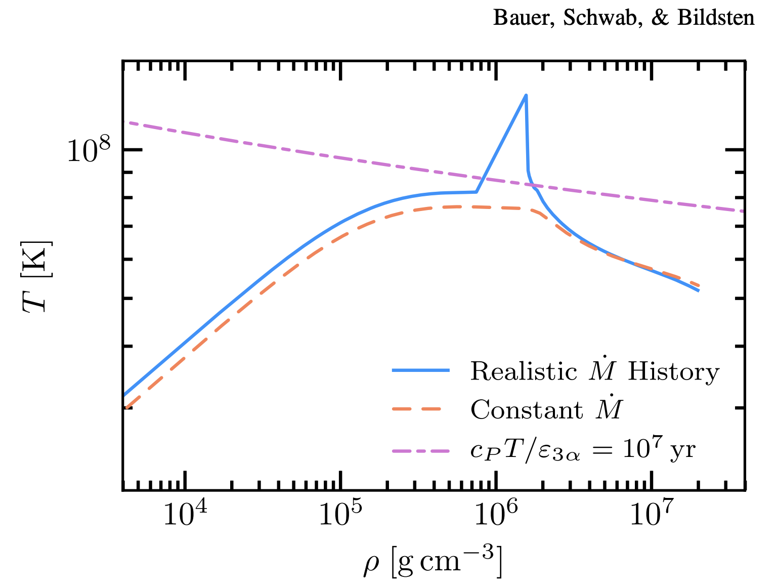
By providing a more accurate accretion history, we have improved the resolution of this ignition feature. This is largely because the rate of accumulation is directly related to the thermal timescale of the accreted material. In other words, changes in accretion rate tie directly to the ability for thermal energy to “escape” from the material with faster accretion deadening this ability. Once this thermal timescale reaches a critical value at the base of this accreted shell, it ignites!
Task 2. Find Helium shell thickness and time to Helium flash
Once the model has completed, copy the procedure from Lab 2 to record Helium shell thickness and time to Helium flash in the Google spreadsheet. Compare these values with the results from Lab 2.
BONUS. Calculating rotation rate of the accretor at Helium flash
Open the history.data log. Use these data to find the rotation rate at the helium flash, assuming the accretor rotates as a solid body. Record this rotation rate in the Google spreadsheet.
We can break this calculation down into three steps. First, find the instantaneous change in angular momentum, J_dot. Then, find the total change in angular momentum, delta_J, up to the Helium flash. Next, find the rotation rate at the Helium flash using the assumed moment of interia, I.
Keep in mind that angular momentum, J, can be expressed as J = sqrt(G * M * R) where G is the graviational constant, M is mass, and R is radius. J in this instance, is the specific angular momentum for Keplerian material at the surface. J_dot should be calculated here assuming that all accreting material deposits that specific angular momentum into the star as it arrives. Hence, we are NOT looking for the Jdot that could be found directly in binary_history.data.
Hint (click here)
Jdot = sqrt(GMR) * Mdot
Hint (click here)
Delta_J = Jdot * s% dt (integrated over time)
Hint (click here)
rotation rate = Delta_J / I
Hint (click here)
The moment of inertia, I, of a solid sphere is (2/5)MR^2