Introduction

So far we have pretended that the accretor will happily accept whatever helium we feed it. However, if mass is dumped onto the accretor surface at a rate faster than heat can be transported, the material is compressed and heats up. It is then possible for the helium layer to reach ignition, leading to a helium flash. Historically, the helium flash is of interest to people modeling type Ia supernova progenitors. If the helium shell is sufficiently thick, during the helium flash, the local heating timescale (timescale to heat a fluid element by nuclear burning) can become shorter than the local dynamical timescale (timescale for sound waves to cross a local pressure scale height), yielding a helium detonation. The helium detonation sends a shock wave into the carbon-oxygen core, and can jump-start detonation of the carbon. This “double-detonation” scenario is one of the many proposed channels for forming a type Ia supernova. In recent years, there has been a lot more focus on double-detonation during a double white dwarf merger (unstable mass transfer), for example see Guillochon+2010.

We will instead take a walk through history and look at double-detonations due to stable mass transfer. The thickness of the helium shell determines whether a detonation is likely. In turn, the thickness of the helium shell is determined by the mass accretion rate. To develop some intuition, we will first consider constant accretion rates. In lab 3 we will connect these to the actual binary donors that you found in lab 1.

Lab Instructions

For this lab we will be running constant mass accretion onto the accretor in single star MESA.

Some helpful links

link to the google spreadsheet of options

link to the github repo (general link)

link to the MESA documentation

Lab 2 solutions if needed –>

Task 0: Download files

Choose your mass and accretion rate from the google spreadsheet of options, then download the correct WD initial accretor model from initial_accretor_models folder in the github repo (direct link to folder).

When you choose your model from the options, think about how the accretion rate you are choosing here compares to the accretion rates you solved for in Lab 1. Are they on the same order of magnitude? Would your binary have been well approximated by a constant accretion rate or was it very different?

Task 1: Generate your inlist

Start by copying the $MESA_DIR/star/work directory to your Lab 2 working directory. Make the following edits to your inlist_project by searching for the appropriate inlist item in the MESA documentation (notice that inlist is only a header file that points to inlist_project and inlist_pgstar).

In star_job:

Turn off pre-main sequence model generation.
We will need to set the code to load in the accretor model that you just downloaded.
We will set the network (change_initial_net) to co_burn.net for this first part.
Set the initial timestep, time, and model number to zero (1d3 in the case of the timestep). Remember you did this in lab 1 as well!
Ensure pgstar output is on (it should be on by default).
Optional (recommended): instruct the model to pause before it terminates so you can view the pgstar output before closing

Hint (click here)

Search for the following in the MESA Documentation: load_saved_model, change_initial_net, set_initial_dt, set_initial_age, pgstar_flag, and pause_before_terminate

In controls:

Turn off the initial mass and initial z that come with the default work directory.
Change the stopping condition. We want to stop when the power generated by helium burning is greater than 10^4 solar luminosities. In other words, we want to put an upper limit on he-burning power at L_He = 10^4 Lsol. (See the hint below if you can’t find the inlist keyword for this)
Turn on the Ledoux criterion.
Add in your constant mass accretion from the spreadsheet (this will be called simply mass_change).

Edit the mesh resolution, adjust the timestep limit, tell the code what to accrete (Mostly Helium in our case!), and update the solver using this code snippet:

! mesh
   mesh_delta_coeff = 1.2d0
! timesteps
   delta_lgL_He_limit = 0.02d0 !0.025d0
! accretion
   xa_function_species(1) = 'he4'
   xa_function_weight(1) = 0 
   xa_function_param(1) = 1d-2
! solver
   energy_eqn_option = 'eps_grav'
   max_resid_jump_limit = 1d20 
   make_gradr_sticky_in_solver_iters = .true.

Hint (click here)

Search for the following in the MESA Documentation: power_he_burn_upper_limit, use_ledoux_criterion, and mass_change

Bonus Task: extra output

As a bonus task, you may choose to add a history column to your output that calculates the thickness of the helium shell as it is accreted. It can be easily calculated after the run is finished, so you will not be in trouble if you don’t complete this task (in other words, do not spend much more than 5 minutes on this!).

Call the new history column he_shell_mass, and it can be calculated in many ways. A few suggestions are star_mass - co_core_mass, star_mass - initial_mass, or mass_change * star_age (remember mass_change is in Msun/yr and star_age is in yrs). The first option contains only variables contained in star_ptr whereas the second two will require you to define a constant value.

Task 2: Inlist pgstar

for your inlist_pgstar:

We have provided a nice inlist_pgstar file in the github repo (direct link to file) which you may download and use. It will contain a nicely formatted pgstar grid for all your viewing needs. Note: Github will interpret this file as a .txt file if you press the download button, which may cause issues. We recommend instead that you copy and paste the text from the block into the inlist_pgstar that comes with the default work directory. If you have any issues loading in this file, please let us know.

You’ll need to adjust a few options within the file:

The first commented chunk will instruct you to change the [plot]_xmin value (in solar masses) for the four plots. You should adjust this value to the mass of your chosen accretor model, but slightly smaller, so that you can monitor the growth of the helium shell.
The second commented chunk has two options to choose between depending on if you did or did not do the previous bonus task (creating the he_shell_mass history column). The default will assume you have not done this bonus task. If you did complete the bonus task, you should switch to the other one. The only difference is that the second one will plot both the accretion rate and the he_shell_mass, and the default option will plot only the accretion rate.

This inlist_pgstar will create a Kippenhahn diagram, which requires an extra step to appear properly. You will need to copy over the history_columns.list defaults (from $MESA_DIR/star/defaults/) and uncomment the mixing_regions <integer> and burning_regions <integer> lines. Replace <integer> in each instance with 20. This number should be large enough that MESA can output the proper amount of boundaries that it needs, however the needed amount is typically small.

Task 3: clean/make/run

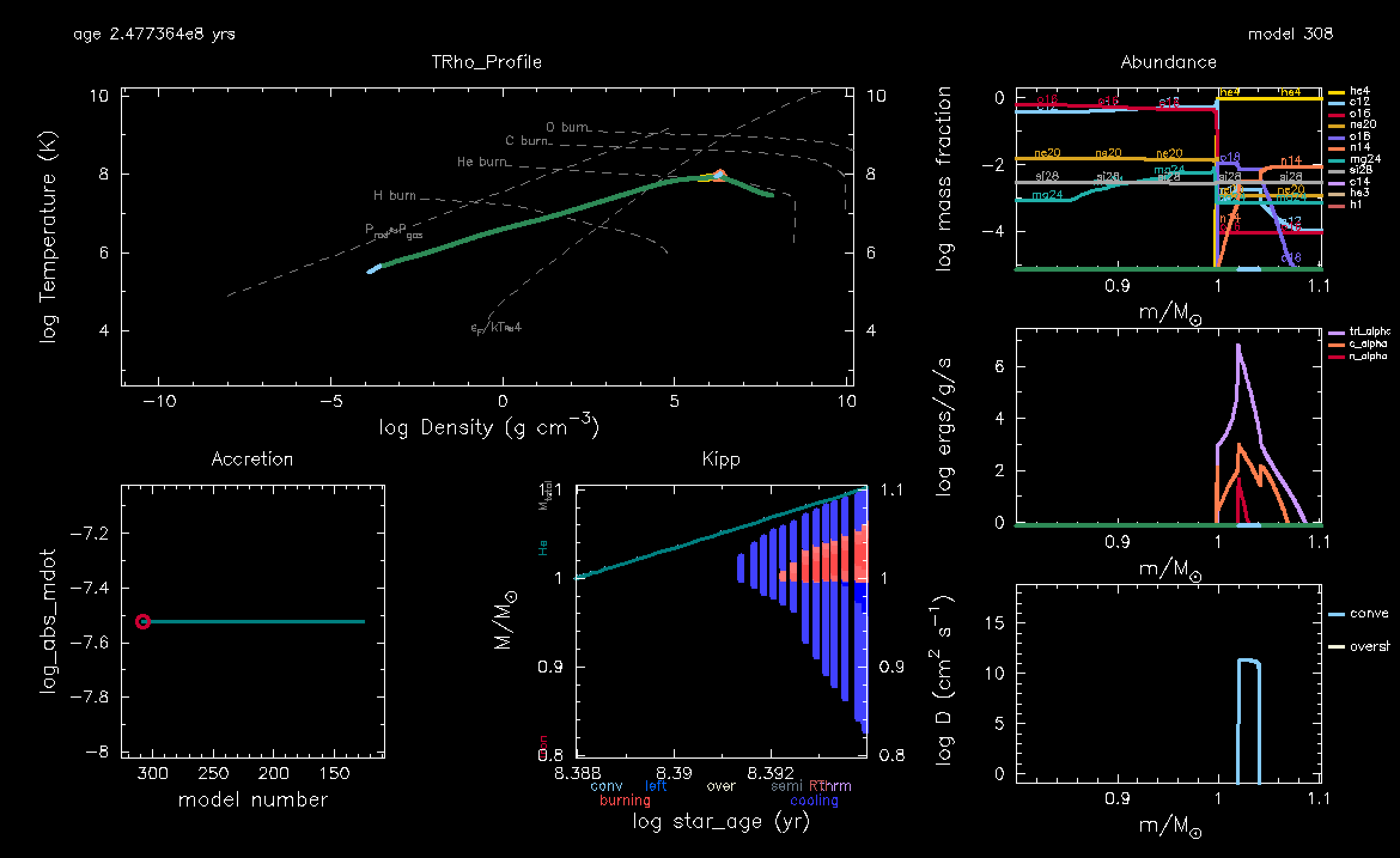
Now go ahead and compile and run your model. At first you should see very little change, but watch the T-Rho diagram. You’ll notice the envelope start to increase in temperature as the accretion heats up the outer layers (this is called compressional heating). You’ll then see a small bump in the T-Rho diagram that will move towards the center of the star. Eventually this bump will increase past the Helium ignition line in the T-Rho diagram and the Power and Kippenhahn plots will begin changing. At this point you should also see the abundance profile changing as Helium rich material is accreted. Your model will terminate soon after ignition. Below is an example of what you should see at the end of a run.

Upon completion of the run, record your helium shell thickness at ignition and the time of helium ignition to the google spreadsheet. Remember that the model will stop running at helium ignition, so this is simply the final values from your history files.

Hint (click here)

The helium shell thickness is star_mass - co_core_mass

A completed run

Task 4: Create a new reaction network

A bit of nucleosynthesis background

Definitions:

The greek letter alpha ($\alpha$) is often used to refer to a Helium nucleus ($^{4}He$), and in MESA will often be referred to as simply a.
The greek letter gamma ($\gamma$) refers to the energy (a photon) generated by a reaction, and in MESA will often be referred to as simply g.
The greek letter nu ($\nu$) refers to a neutrino, and reactions using this are often referred to as “weak” reactions.
The letter $n$ refers to a neutron, and in MESA will often be referred to as neu or n.
We will use $e^-$ to refer to electrons, and in MESA this is usually e.
Isotopes are referred to with the notation $^{\#}X$ where X is the chemical symbol and # is the mass number. However, in MESA internals, these are usually referred to more simply as x#. As an example, the Carbon-12 isotope can be written as $^{12}C$, but in MESA it will be called c12.

Finally, we will use reaction notation in the instructions. If you are unfamiliar, it is a compact notation used to describe nuclear reaction. Reactions which we might normally write as:

\[A + b \rightarrow D + c\]

You could then write more compactly as:

\[A(b,c)D\]

So as an example, the following alpha-capture reaction on $^{12}C$ to create $^{16}O$ and energy:

\[^{12}C + \alpha \rightarrow ^{16}O + \gamma\]

is equivalently written as:

\[^{12}C(\alpha,\gamma)^{16}O\]

In general, MESA doesn’t use a standard notation for reactions, but in the networks there will usually be a comment explaining exactly which reaction they mean if there is any ambiguity. In the case of this particular reaction, MESA calls it r_c12_ag_o16.

The actual task

Now, we will run the same inlists but with a new reaction network of our creation. We will generate our own reaction network that includes the “NCO” reaction chain ($^{14}N(e^-,\nu)^{14}C(\alpha,\gamma)^{18}O$) and also adjust the reaction rate for $^{14}C(\alpha,\gamma)^{18}O$.

There is detailed network documentation in the MESA Docs which you may refer to throughout this section for more details

Up until now we have been using the reaction network called co_burn.net. Navigate to $MESA_DIR/data/net_data/nets to view the source files for all of the available reaction networks. Start by opening co_burn.net and viewing its contents. You’ll see that it contains very little information, and instead points to two other files. Open and examine those other files. You’ll see that these other two files have much more information in them. Refer to the docs to see how the functions add_isos() and add_reactions() work.

Recommended: If you’d like for your MESA run to print out its net information at start (for example to check if it’s implementing your new reactions!), you can add the following to the star_job section of your inlist:

show_net_species_info = .true. ! to list all of the isotopes in the net
show_net_reactions_info = .true. ! to output information on all net reactions
list_net_reactions = .true. ! to output a simple list of all the reactions in your net

Now lets generate our own reaction network. Begin by copying co_burn.net to your lab 2 working directory and giving it a new name, something like nco.net. Decide which isotopes you’ll need to add in for the NCO reaction, either by examining co_burn.net and its constituent files or by outputting the net data to the terminal. Add those isotopes to the reaction network using add_isos_and_reactions(). This will automatically add all reactions associated with those isotopes as well.

Hint (click here)

The two isotopes you will need are c14 and o18

Make sure to change your inlist_project to take in nco.net as the reaction network, rather than co_burn.net! Note that mesa will search for reaction networks in your working directory as well as in $MESA_DIR/data/net_data/nets to find the network you call here.

Now we’ll update the reaction rate for $^{14}C(\alpha,\gamma)^{18}O$. Download the zip file called tables_hashimoto.zip from the github repo (direct link to zip). Once you unzip this file, there will be a folder called tables_hashimoto which you should place inside your Lab 2 work directory. Now add the following section to the star_job section of your inlist:

  ! adjusting nuclear reaction rates
    rate_tables_dir = 'tables_hashimoto'
    rate_cache_suffix = 'hashimoto'

These tables are called such as they come from Hashimoto+ 1986. The weak rates were provided by Gabriel Martínez-Pinedo and used in Bauer+ 2017.

If you look inside the file tables_hashimoto/rate_list.txt you will see this:

! this is an example of a rates list file for use with mesa/rates
! the mesa/data/net_data/rates directory has sample rate files
! pairs of rate name and rate file

r_c14_ag_o18   'c14rate_Hashimoto_reduced.txt'

The last line here indicates that the rate for the $^{14}C(\alpha,\gamma)^{18}O$ reaction will be read from a file called c14rate_Hashimoto_reduced.txt which also lives in the folder called tables_hashimoto. Opening this file will reveal a simple two column file (columns correspond roughly to temperature and rate) that MESA will read to load the new reaction rates. You may also inspect tables_hashimoto/weak_rate_list.txt which works similarly. See the documentation for further info.

STOP
Did you change your reaction network to the one you just made?

Task 5: clean/make/run

Recompile and run your new model. When you run this model, if you’ve chosen to output your net data, it would be good to check that you are properly including your newly added elements. If you have not output net data, you can check the abundance panel in the pgstar output to see if there is a line for $^{18}O$ that appears.

Upon the run’s completion, record your helium shell thickness and the time of helium ignition to the google spreadsheet.

As everyone finishes their models, we can ask: how does the Helium shell thickness at ignition vary with accretion rate and accretor mass, and how does changing the reaction networks change these values?

Lab Extension (over lunch)

Expected Runtime: ~30 minutes on 4 cores

If you would like to view what happens after helium ignition, you can turn off the stopping condition in the inlist and allow your model to run over lunchtime. You will see very interesting things happening in your T-Rho diagram! If you haven’t, we highly recommend adding pause_before_terminate = .true. to the star_job section of inlist_project so that you can view the pgstar output when you return from lunch. Below is a video of what you should see, in case you decide not to run this.

Solutions

If you need any solutions for Lab 2: you can find them here

Back to main page